Data Transformations: Log, Square Root, and Box-Cox Without Guesswork

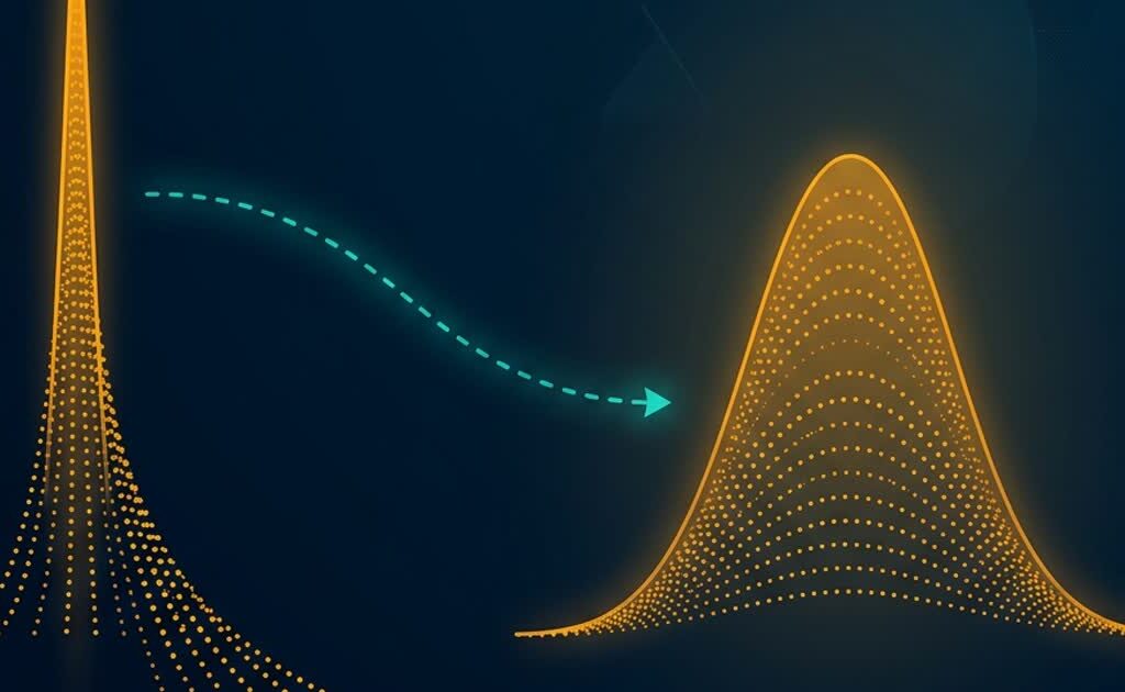
Income, viral load, reaction time, bacterial counts, hospital length of stay. Each is positive, each is skewed, and each will produce residuals that fan out and a normality test that fails. The traditional response is to transform the variable until the model behaves.

Transformation is a legitimate and powerful tool, but it changes the question being answered as well as the scale. Applying one reflexively, or back-transforming carelessly, produces conclusions that are precise and wrong.

What a transformation can and cannot fix

A transformation changes the shape of a distribution. It can reduce skew, stabilise variance, and linearise a curved relationship. It cannot add information, remove confounding, or make a badly designed study interpretable.

Problem	Transformation helps?	Better alternative sometimes
Right-skewed positive outcome	Yes, log or Box-Cox	Gamma GLM
Variance grows with the mean	Yes, variance-stabilising	Weighted least squares, robust SEs
Curved relationship	Yes, if the curve is of the right family	Polynomial or spline term
Counts with many zeros	No, log is undefined at zero	Poisson, negative binomial, hurdle
Proportions at 0 or 1	No, logit is undefined at the bounds	Beta or binomial regression
Measurement error	No	Nothing statistical helps

The log transformation

Logarithms compress large values and expand small ones, converting multiplicative relationships into additive ones. That is why they dominate in biology, economics and epidemiology, where effects are naturally proportional rather than absolute.

The interpretive consequence is the important part. On a log scale a coefficient is a difference in logs, which exponentiates to a ratio. A coefficient of 0.09 on a log scale means roughly a 9% increase per unit of the predictor — a proportional change, constant across the range, rather than a fixed number of units.

# R
dat$log_income <- log(dat$income)          # natural log
fit <- lm(log_income ~ education + region, data = dat)

# proportional interpretation
exp(coef(fit)) - 1                          # percent change per unit

# Python
import numpy as np
import statsmodels.formula.api as smf

dat["log_income"] = np.log(dat["income"])
fit = smf.ols("log_income ~ education + region", data=dat).fit()
np.exp(fit.params) - 1

Zeros are the practical obstacle. log(0) is undefined, and adding a constant — log(x + 1) — is a different transformation whose results depend on the constant chosen. It is defensible for counts where a one-unit shift is meaningful, and dubious elsewhere. If the zeros are real and numerous, a count model is the honest route.

Note the units: a natural log and a base-10 log differ by a constant factor of about 2.30, so coefficients are not comparable across the two unless you convert. State which base you used.

Square roots and reciprocals

The square root is the variance-stabilising transformation for Poisson-like counts: if the variance grows with the mean, the variance of the square root is roughly constant. It handles zeros gracefully, since the square root of zero is zero, which is why it remains popular for counts that no longer fit well in a count model.

dat$sqrt_count <- sqrt(dat$count)
fit <- lm(sqrt_count ~ treatment + block, data = dat)

The reciprocal is the transformation for rates and times: if Y is time per unit, then 1/Y is units per time, which is often the quantity that behaves linearly. It is rarely interpretable on its own terms and should be used only when the reciprocal has a clear physical meaning.

Choosing a power rather than guessing

Log, square root, reciprocal and identity are all members of one family: the Box-Cox power transformation, indexed by a single parameter. Box-Cox estimates that parameter by maximum likelihood, which turns a judgement call into an estimable quantity.

Estimated λ	Transformation	Typical use
1	None (identity)	Already well behaved
0.5	Square root	Counts, mild right skew
0	Natural log	Multiplicative effects, strong right skew
-0.5	Inverse square root	Rates
-1	Reciprocal	Times and rates

# R
library(MASS)
bc <- boxcox(lm(y ~ x, data = dat), lambda = seq(-2, 2, 0.05))
lambda <- bc$x[which.max(bc$y)]

# or, with a confidence interval
car::powerTransform(lm(y ~ x, data = dat), family = "bcPower")
summary(car::powerTransform(lm(y ~ x, data = dat)))

# Python
from scipy import stats
y_transformed, lam = stats.boxcox(dat["y"].values)
print(lam)

Box-Cox requires strictly positive values. For data containing zeros or negatives, Yeo-Johnson extends the same family to the whole real line, at the cost of a slightly less intuitive interpretation.

car::powerTransform(lm(y ~ x, data = dat), family = "yjPower")

Two cautions. The estimate is sensitive to outliers, so check the diagnostics before trusting the λ. And a λ estimated at 0.07 is practically a log transformation; rounding to a familiar power usually costs nothing and makes the result far easier to explain.

The back-transformation trap

Fitting a model on a log scale and then exponentiating the predicted value gives the median, not the mean. The mean of logged values exponentiates to the geometric mean, which is always smaller than the arithmetic mean when the data are skewed. If you report a mean in the original units, this matters.

# R: the naive and the corrected back-transformation
naive <- exp(mean(log(dat$y)))
corrected <- exp(mean(log(dat$y)) + var(log(dat$y)) / 2)   # lognormal mean

For regression predictions the correction is the smearing estimator: average the exponentiated residuals and multiply. Reporting the geometric mean is often the better choice anyway, provided you name it as such — a geometric mean of viral load is a meaningful quantity, and calling it the mean is the error.

Confidence intervals are easier: compute them on the transformed scale, where they are symmetric, then exponentiate both limits. The result is asymmetric in the original units, which is correct and should not be straightened out.

When not to transform

Three situations argue against transformation even when it would improve the diagnostics.

• Interpretability dominates. A coefficient in log-days of hospital stay may be statistically cleaner and practically opaque.
• The outcome is a count or a proportion with structural zeros, where a generalised linear model encodes the mean-variance relationship properly instead of approximating it.
• The goal is prediction rather than explanation. A model on a transformed scale optimises error in transformed units, which is rarely the loss function you care about.

Modern practice increasingly prefers a GLM with an appropriate link over a transformed outcome, because the model states its assumptions about the variance instead of hiding them in an algebraic change of scale. The trade-off is that GLM coefficients are on a link scale too, so interpretation requires the same care.

What to report

Name the transformation, state the base for logs, give the estimated power and its confidence interval if one was estimated, report the diagnostics before and after, and be explicit about what the reported estimate means in the original units. If a mean was back-transformed, say whether it is an arithmetic mean, a geometric mean, or a corrected estimate.

Transformations are one of several ways to make a model fit the data, alongside robust estimation and generalised linear models, and choosing among them is a modelling decision worth defending. Ampersand Academy covers those alternatives with worked examples.

Practice

1. Plot a skewed variable before and after a log transformation and compare the residual patterns from both models.
2. Estimate λ by Box-Cox, then refit with the rounded value and report whether the fit changed materially.
3. Compute the arithmetic mean, the geometric mean, and the corrected mean of the same skewed variable.
4. Argue for or against a GLM alternative in three sentences, naming the assumption each approach makes.

Related tutorials

• Checking Statistical Assumptions in Practice: What to Plot, What to Trust, What to Do Next — the diagnostics a transformation is meant to improve
• ANOVA and Post-Hoc Tests: Comparing Three or More Groups Properly — comparing groups when the outcome is multiplicative
• Distributions in Statistics: Types with Examples — the distribution shapes each transformation targets