Time Series Analysis: Autocorrelation, ARIMA, and Why Random Splits Fail

Daily case counts, monthly sales, hourly sensor readings. The rows are in an order that matters, and that single fact invalidates most of the default machinery you would reach for: a regression that assumes independent errors, and cross-validation that shuffles rows at random.

Time series analysis is mostly about respecting that ordering. The methods are not exotic — differencing, autocorrelation functions, ARIMA, rolling validation — but each one exists to handle a specific consequence of dependence.

Why ordinary regression fails on ordered data

Standard regression assumes independent errors. In time series, consecutive values are almost always related: a high value today makes a high value tomorrow more likely. Residuals from such a series are autocorrelated, which breaks the assumption behind every standard error.

The practical consequence is that confidence intervals become far too narrow and p-values far too small. A covariate that is merely trending upward alongside your outcome will appear overwhelmingly significant, because both series drift and the model has no way to tell drift from relationship.

Assumption	What breaking it does
Independent errors	Understated standard errors, inflated significance
Constant variance	Heteroscedastic periods distort intervals
No trend in residuals	Spurious regression between unrelated trending series
Random validation split	Leakage; optimistic error estimates

Autocorrelation: measuring dependence

The autocorrelation function shows the correlation between the series and its own lagged values. Plot it first, before fitting anything — the ACF and its partial counterpart (PACF) tell you what structure the model needs.

# R
library(forecast)
Acf(daily_counts,  lag.max = 40)
Pacf(daily_counts, lag.max = 40)

# Python
from statsmodels.graphics.tsaplots import plot_acf, plot_pacf
plot_acf(series, lags=40)
plot_pacf(series, lags=40, method="ywm")

Reading them takes a little practice. A slowly decaying ACF suggests a trend or a need to difference. A spike at lag 12 in a monthly series indicates seasonality. A sharp cutoff in the ACF after lag q with a gradual PACF decay is the signature of a moving-average component, and the reverse pattern suggests an autoregressive one.

Durbin-Watson is the quick numeric check for residual autocorrelation in a regression: values near 2 are reassuring, values well below 2 mean positive autocorrelation, and the usual response is to model the dependence rather than ignore it.

library(lmtest)
dwtest(model)          # residual autocorrelation in a regression

Decomposition: separate the parts

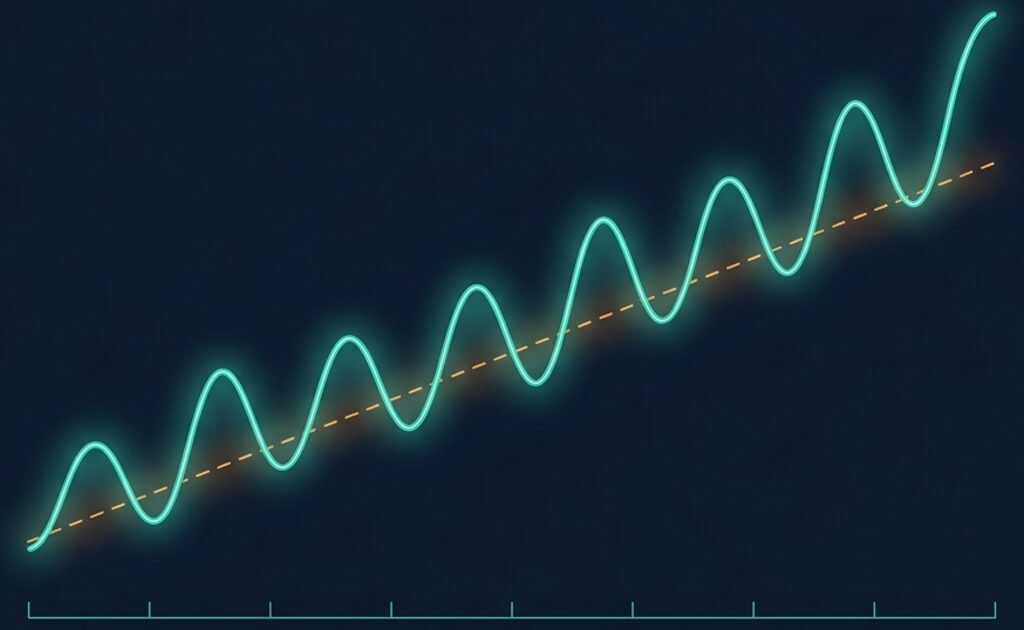
A time series is usually a mix of trend, seasonal pattern, and irregular remainder. Decomposing makes each visible, and the choice between additive and multiplicative matters: with an additive model the seasonal swing is a constant size, with a multiplicative model it grows as the series grows.

decomp <- stl(daily_counts, s.window = "periodic")
plot(decomp)
decomp$time.series[1:5, ]

Look at the remainder panel. If what is left over still shows structure — a wave, a level shift, a growing variance — the decomposition has not captured the whole story and a model built on it will carry that structure into its residuals.

Stationarity and differencing

ARIMA models assume stationarity: constant mean, constant variance, and autocorrelation structure that depends only on lag, not on time. Real data rarely satisfy this, so you transform until it does — usually by differencing.

# R
checkresiduals(auto.arima(daily_counts))   # not a stationarity test, but useful
library(tseries)
adf.test(daily_counts)                     # unit root test
kpss.test(daily_counts)                    # opposite null: stationarity

# Python
from statsmodels.tsa.stattools import adfuller
adfuller(series, autolag="AIC")

The two tests have opposite null hypotheses, and using both is more informative than trusting either alone: ADF rejects a unit root, KPSS rejects stationarity. If ADF fails to reject and KPSS rejects, difference the series. If both pass, you are probably fine. If they disagree confusingly, look at the plot rather than running a third test.

diff1 <- diff(daily_counts, differences = 1)
diff2 <- diff(daily_counts, differences = 1, lag = 12)   # seasonal differencing

Do not difference more than necessary. Overdifferencing introduces artificial negative autocorrelation at lag one and inflates variance, which is why automated order selection should be sanity-checked against the plots.

ARIMA in practice

ARIMA(p, d, q) combines an autoregressive part, the number of differences, and a moving-average part. The seasonal extension adds one of each at the seasonal period. Choosing orders by eye from ACF and PACF is traditional; choosing them by information criterion is more reproducible.

# R: automatic selection, then check it
fit <- auto.arima(daily_counts, seasonal = TRUE,
                  stepwise = FALSE, approximation = FALSE)
summary(fit)
checkresiduals(fit)          # Ljung-Box on the residuals
forecast(fit, h = 14) |> plot()

# Python
from statsmodels.tsa.statespace.sarimax import SARIMAX
model = SARIMAX(series, order=(1, 1, 1), seasonal_order=(1, 1, 0, 12),
                enforce_stationarity=True, enforce_invertibility=True)
res = model.fit(disp=False)
print(res.summary())
res.plot_diagnostics(figsize=(10, 8))

checkresiduals is the step people skip. If the residuals still show autocorrelation in the ACF or a significant Ljung-Box test, the model has not captured the dependence and the forecast intervals will be wrong even if the point forecasts look reasonable.

Two honest boundaries. ARIMA is a linear model and will not capture regime changes or volatility clustering — for the latter, GARCH-family models exist. And a forecast interval that widens slowly is only trustworthy if the residuals are genuinely white noise.

Lagged effects and cross-correlation

If you have an intervention or a second series, the question is usually whether one leads the other. Prewhitening both series before computing cross-correlation avoids the classic trap where two independently trending series appear strongly related at every lag.

ccf(prewhiten(x), prewhiten(y), lag.max = 12, plot = TRUE)

An apparent peak at lag 3 in raw cross-correlations often disappears once both series are prewhitened. If it survives, that is a lagged association worth modelling.

Validation: random splits do not work

Shuffling rows and cross-validating leaks future information into training, producing error estimates that look excellent and forecasts that disappoint. Validation must respect time: train on the past, test on the future.

# Rolling-origin evaluation
n <- length(daily_counts)
train <- window(daily_counts, end = n - 30)
test  <- window(daily_counts, start = n - 29)
accuracy(forecast(auto.arima(train), h = 30), test)

One holdout is better than a random split but still a single sample. Rolling-origin evaluation — repeatedly refitting and forecasting further ahead — gives a distribution of errors across regimes, which is what you need to state expected performance honestly.

# tsCV: rolling origin, one-step ahead
e <- tsCV(daily_counts, forecastfunction = function(y, h) {
  forecast(auto.arima(y), h = h)
}, h = 1)
sqrt(mean(e^2, na.rm = TRUE))     # rolling RMSE

Validation scheme	Use when
Random k-fold	Never for temporal data
Single holdout, last period	Quick sanity check
Rolling origin (walk-forward)	Standard for forecasting performance
Block bootstrap	Uncertainty intervals for dependent series

Report a baseline too. A naive forecast — yesterday’s value, or the same period last season — is embarrassingly hard to beat, and a model that cannot beat it adds complexity without value.

accuracy(snaive(daily_counts, h = 14))    # seasonal naive baseline

What to report

Give the frequency and the period covered, the transformation and differencing applied, the model orders and how they were chosen, residual diagnostics including the Ljung-Box result, the validation scheme with its error metric, and a naive baseline for comparison. State the forecast horizon explicitly, because accuracy degrades with horizon and one number cannot describe both.

Respecting dependence is a design principle that shows up across statistics, from repeated measures to clustered samples. If you want to see how the same idea is handled in other designs, Ampersand Academy covers the family of methods built for dependent data.

Practice

1. Plot the ACF and PACF of a series with a clear trend and describe what each suggests.
2. Compare ADF and KPSS on the raw and differenced series and decide how many differences are needed.
3. Fit an ARIMA model, run residual diagnostics, and report the Ljung-Box result.
4. Compare rolling-origin RMSE against a seasonal naive baseline and state whether the model earns its complexity.

Related tutorials

• Bootstrapping and Resampling: Confidence Intervals Without Distributional Assumptions — block resampling for dependent observations
• Correlation Coefficient: How to Read r Correctly — reading associations when the data are ordered in time
• Checking Statistical Assumptions in Practice: What to Plot, What to Trust, What to Do Next — residual diagnostics as assumption checking