Survival Analysis: Kaplan-Meier Curves and Cox Regression, Worked Through

A study follows patients for five years and records when each one dies, relapses or is discharged. Halfway through, some participants move away; others are still healthy when the funding ends. You know only that they survived at least until their last observation. This is censoring, and it is what makes time-to-event data a different statistical problem rather than a t-test with a stopwatch.

Survival analysis exists to use that partial information properly. Ignoring censored subjects biases survival downward; dropping them biases it upward. Neither is acceptable, and both are common in drafts that reach reviewers.

Why time-to-event data breaks ordinary statistics

Three features make standard methods fail.

• The outcome is not just whether the event happened, but when — so a single proportion throws away the timing that is the whole point.
• Observations are incomplete in a specific, informative way: right-censored subjects contribute time but no event.
• Risk is not constant over time. The hazard of an event in month one is rarely the hazard in month forty-eight.

If you analysed this with a plain logistic regression on ever/never, you would silently assume that everyone followed for one day and someone followed for five years carries equal information. That is why survival methods weight each event by how many people were still at risk at that moment.

Censoring, precisely

Right censoring means the event happened after the last observation, or was never observed. It is uninformative only if the reason for censoring is unrelated to prognosis — someone relocating for work is fine; someone dropping out because they felt too ill is not, and that is informative censoring, which no standard method repairs.

Type	What you observe	Consequence
Event	Exact time of event	Full information
Right-censored	Survived until time t, outcome unknown after	Handled by KM and Cox
Left-censored	Event occurred before t	Needs specialised methods
Interval-censored	Event between two visits	Needs interval methods; KM is biased

Interval censoring is the one people miss. If patients are seen annually, the true event time is somewhere in a twelve-month window, and pretending it happened at the visit date biases the curve. If your data are visit-based, say so.

Kaplan-Meier: what the curve is doing

The Kaplan-Meier estimator multiplies conditional survival probabilities across every event time. At each event, survival drops by the fraction of those still at risk who experienced it. Subjects censored before that point leave the risk set without causing a drop, which is exactly the correction ordinary proportions lack.

library(survival)

fit <- survfit(Surv(time, event) ~ group, data = trial)
summary(fit)              # survival at each event time
summary(fit, times = c(12, 36, 60))   # survival at chosen timepoints

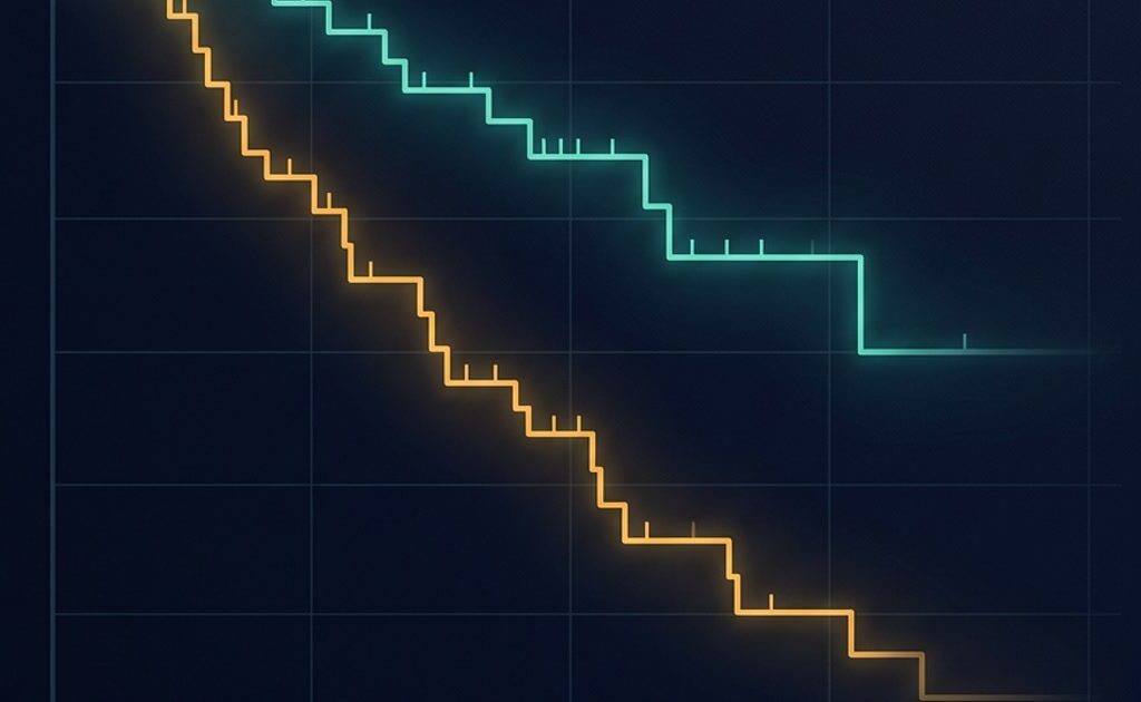
Reading it correctly takes three habits. First, the curve is a step function, not a smooth trend — it changes only at event times. Second, the number at risk falls over time, so the right-hand end of a curve is estimated from very few people and is correspondingly uncertain. Third, the curve never reaches zero unless every subject had the event.

Confidence bands and the tail

The shaded band is a pointwise confidence interval, which is not a simultaneous band: the chance that the whole curve lies inside it is lower than 95%. Near the end of follow-up the band widens dramatically because the risk set has shrunk. Truncating curves at a stated median follow-up, with numbers-at-risk printed beneath, is standard practice precisely because it prevents the misleading tail.

library(survminer)
ggsurvplot(fit, data = trial, risk.table = TRUE,
           conf.int = TRUE, xlim = c(0, 60),
           break.time.by = 12,
           legend.title = "Group")

The risk table is not decoration. A curve that separates only after month 48, when twelve people remain at risk, is a very different claim from one that separates at month 6 with 300 at risk — and the table is how a reader tells which they are looking at.

The log-rank test, and its one job

The log-rank test compares entire survival curves between groups. It asks whether the observed number of events in each group differs from what you would expect if survival were identical, summed across all event times.

survdiff(Surv(time, event) ~ group, data = trial)

It is a test of the whole curve, not of any single timepoint, and it has low power when curves cross. If one treatment is better early and worse later, the log-rank test can return a large p-value while both directions matter clinically. In that case report the curves, consider a time-varying or restricted-mean analysis, and do not claim equivalence.

Cox regression and hazard ratios

Cox proportional hazards models the hazard — the instantaneous risk of the event given survival so far — as a baseline hazard multiplied by an exponential function of the covariates. The baseline hazard is left unspecified, which is why it is called semi-parametric and why it is so widely used.

cox <- coxph(Surv(time, event) ~ treatment + age + stage, data = trial)
summary(cox)
exp(coef(cox))              # hazard ratios
exp(confint(cox))           # 95% CI

A hazard ratio of 0.72 for treatment means: at any given moment, among those still at risk, the treated group’s instantaneous risk is 72% of the control group’s. It does not mean 28% fewer events overall, and it does not mean a 28% longer survival time. Converting a hazard ratio into a difference in median survival requires the baseline hazard, which is why those two numbers rarely match.

Statement	Correct?
Treated patients had 28% lower hazard at any given time	Yes
Treated patients were 28% less likely to have the event	No — that needs absolute risks
Median survival was 28% longer	No — HR and median ratio differ
The treatment delayed events proportionally	Only if proportional hazards holds

The proportional hazards assumption

Cox regression assumes the hazard ratio is constant over time. If treatment helps most in the first six months and not afterwards, the model averages two different realities into one number. This assumption is testable and routinely untested.

cox.zph(cox)                # Schoenfeld residuals test
plot(cox.zph(cox))          # look for a trend, not just the p-value

A significant result means the proportional hazards assumption is doubtful — but the test is sensitive with large samples and underpowered with small ones, so inspect the plot too. When the assumption fails, the standard options are stratification on the offending variable, a time-varying coefficient, an interaction with time, or reporting separate hazard ratios for prespecified periods.

# Stratify by stage rather than modelling it proportionally
cox_strat <- coxph(Surv(time, event) ~ treatment + age + strata(stage), data = trial)

Competing risks

If patients can die of something unrelated before the event of interest, a standard Kaplan-Meier curve overestimates the incidence of the event, because it treats death as censoring rather than as a competing outcome that removes the possibility of the event. Cumulative incidence functions are the right tool, and the difference becomes material in older populations.

# Cumulative incidence with competing risks
library(cmprsk)
cuminc(trial$time, trial$status, trial$group)

What to report

Report the number of events, not just the sample size — power in survival analysis is driven by events. Give median follow-up with its method, curves truncated at a defensible time with numbers at risk, hazard ratios with confidence intervals, the proportional hazards check, and explicit mention of any competing risks. Avoid reporting a hazard ratio without stating whether the assumption held.

Time-to-event reasoning connects directly to study design: how many events you need, and how long you must follow people to get them. If you want to build that planning skill properly, Ampersand Academy covers the design-to-analysis sequence.

Practice

1. Plot a Kaplan-Meier curve with the risk table and state the median follow-up rather than the maximum.
2. Run the log-rank test, then describe a scenario where it would mislead.
3. Fit a Cox model, interpret one hazard ratio in a sentence that does not mention probability of the event.
4. Test proportional hazards and try one remedy if the assumption fails.

Related tutorials

• Repeated Measures Are Not Independent: When to Use Mixed Models — the other family of models for clustered observations
• Checking Statistical Assumptions in Practice: What to Plot, What to Trust, What to Do Next — how to test the proportional hazards assumption rather than assume it
• How to Choose a Sample Size: Power Analysis That Does Not Lie to You — planning an event-driven study before you collect a single sample