Bayesian Statistics: Priors, Posteriors, and Credible Intervals Explained

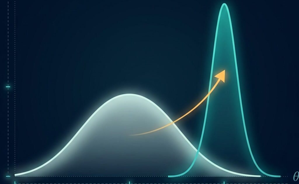
The frequentist question is: if this experiment were repeated endlessly, how often would I see a result this extreme? The Bayesian question is more direct: given what I observed, what should I believe about the effect? For most people asking a research question, the second is what they actually want, and they have been trained to answer the first.

Bayesian statistics is not a different kind of arithmetic; it is a different statement about what probability means. A parameter — a true effect size, a conversion rate — is treated as unknown but describable by a distribution, rather than as a fixed constant that only sampling distributions can illuminate.

What changes when you treat parameters as uncertain

Bayes’ theorem combines two things: what you believed before seeing data, and how well the data support each possible value. The result is a posterior distribution — a full description of your uncertainty about the parameter after observing the data.

posterior  ∝  likelihood  ×  prior

That single line is the whole method. The likelihood is the same object a frequentist uses. The prior is the addition, and it is the source of both the method’s power and its reputational problem.

Quantity	Frequentist	Bayesian
Parameter	Fixed unknown constant	Random variable with a distribution
Probability means	Long-run frequency	Degree of belief
Inference from	Sampling distribution	Posterior distribution
Interval	Confidence interval	Credible interval
Optional stopping	Inflates error rates	Posterior updates coherently
Prior information	Not formally used	Explicit and required

Priors: the part that needs defending

A prior is a probability distribution over the parameter before seeing data. There is no prior-free Bayesian analysis, only priors whose influence is hidden, so the honest move is to state one and show that the conclusion does not hinge on it.

Prior type	Example	When it is appropriate
Flat / reference	Uniform on a bounded range	Little prior knowledge; check it is not inadvertently informative
Weakly informative	Normal(0, 1) on a log-odds scale	A sensible default that keeps estimates in a plausible range
Regularising	Half-normal on a standard deviation	Prevents degenerate fits; standard in Stan and brms
Informative	Based on previous trials, with justification	Strong prior evidence exists and you can cite it

Two practical notes. First, a flat prior is not neutral: on a transformed scale it implies information about the original scale, so a uniform prior on a probability is not uniform on its log-odds. Second, weakly informative priors are usually the best default — they rarely change a well-powered conclusion, and they stabilise a poorly-powered one instead of letting the likelihood run to infinity.

Priors help most when data are sparse

With a large sample the likelihood dominates and the prior barely matters. With twelve observations, a separating predictor, or a rare event, the prior is doing real work — and that is exactly the situation where stating it is most important.

The posterior is the answer

Everything you want comes from the posterior distribution: the most likely value, an interval containing 95% of the posterior mass, and the probability that the effect exceeds a threshold of interest. That last one has no clean frequentist equivalent and is often what a decision-maker wants.

# R: brms wraps Stan for regression models
library(brms)

fit <- brm(responded | trials(n) ~ treatment + age,
           family = binomial(),
           data = trial,
           prior = c(prior(normal(0, 1.5), class = "b"),
                     prior(normal(0, 2), class = "Intercept")),
           chains = 4, iter = 2000, seed = 42)

summary(fit)
posterior_interval(fit, prob = 0.95)

# Python: PyMC for a two-group comparison
import pymc as pm

with pm.Model() as model:
    mu_a = pm.Normal("mu_a", 0, 1)
    mu_b = pm.Normal("mu_b", 0, 1)
    sigma = pm.HalfNormal("sigma", 1)
    pm.Normal("a", mu_a, sigma, observed=group_a)
    pm.Normal("b", mu_b, sigma, observed=group_b)
    diff = pm.Deterministic("diff", mu_b - mu_a)
    trace = pm.sample(2000, tune=1000, chains=4, random_seed=42)

pm.plot_posterior(trace, var_names=["diff"])

Direct probability statements

# How much posterior mass says the effect is meaningfully positive?
post <- as_draws_df(fit)
mean(post$b_treatment > 0.2)

That line returns something like 0.94, which reads exactly as it sounds: a 94% posterior probability that the effect exceeds 0.2. Compare with a p-value, which is neither the probability the null is true nor the probability the result would replicate.

Credible intervals versus confidence intervals

These two intervals look identical on a page and mean different things. A 95% confidence interval is a statement about the procedure: intervals built this way capture the true value in 95% of repeated experiments. It says nothing about the specific interval you calculated.

A 95% credible interval is a statement about the parameter, given your data and prior: there is 95% posterior probability that the parameter lies in this range. That is what nearly everyone assumes a confidence interval means, which is a large part of the Bayesian method’s appeal.

Statement	Confidence interval	Credible interval
95% refers to	The procedure over repeated samples	The posterior mass for this parameter
Requires a prior	No	Yes
Valid with one dataset	Interpretation is indirect	Direct probability statement
Shrinks with stronger prior	Not applicable	Yes — for better or worse

There is also a subtlety inside the Bayesian world: the equal-tailed interval takes 2.5% from each tail, the highest-density interval takes the narrowest 95% region. For skewed posteriors they differ, and you should say which you used.

Bayes factors, and the null-result problem

A Bayes factor compares the evidence for two models — typically an effect model against a null model. Unlike a p-value it can support the null, which is why it appears in equivalence and replication work.

The catch is sensitivity to the prior on the effect size, which is precisely the parameter you are trying to judge. Different reasonable priors can move the Bayes factor by an order of magnitude, so a Bayes factor reported without its prior specification is not interpretable. Present a sensitivity analysis across a few defensible priors.

Bayes factor (H1 vs H0)	Loose reading
Below 1/10	Strong evidence for the null
1/3 to 1	Weak evidence for the null
1 to 3	Barely worth mentioning either way
3 to 10	Moderate evidence for the effect
Above 30	Strong evidence for the effect

Where the method genuinely pays off

• Multilevel data: partial pooling gives small groups shrunk toward the overall mean, which is exactly right and hard to do elegantly elsewhere.
• Small samples and sparse events, where a weakly informative prior prevents absurd estimates.
• Sequential data: you can look at accumulating evidence and update without the error inflation of repeated significance testing.
• Direct probability statements for decisions, such as the probability a treatment is cost-effective.
• Missing data handled jointly with the model rather than in a separate imputation step.

The practical objections, honestly

Computation is no longer a barrier — Stan, PyMC and brms fit most applied models in minutes. The real costs are these: you must specify and defend a prior, convergence diagnostics need checking (R-hat, effective sample size, divergences), and reviewers trained in frequentist methods may ask for a p-value anyway.

# Diagnostics that are not optional
summary(fit)$fixed          # check Rhat close to 1.00
plot(fit)                   # trace and posterior plots
# Divergent transitions in the sampler output mean the fit is unreliable

A common and defensible compromise is to run the analysis both ways. When a weakly informative Bayesian model and a frequentist model agree, the prior is not driving your conclusion, and that agreement is worth stating explicitly.

What to report

Give the model, the likelihood, every prior with its justification, the posterior estimates with credible intervals and the interval type, the convergence diagnostics, and a prior sensitivity check. If you report a Bayes factor, report the priors it was computed under and how the value changes across them.

The conceptual shift — expressing uncertainty about a parameter rather than about a procedure — is worth understanding regardless of whether you adopt the toolchain, because it clarifies what a confidence interval was always trying to say. Ampersand Academy walks through that reasoning with worked examples.

Practice

1. Fit a simple two-group model with a weakly informative prior and with a deliberately strong one; compare the posteriors.
2. Report the posterior probability that the effect exceeds a meaningful threshold, not just the interval.
3. Compute a Bayes factor under three different priors and describe how much the conclusion moves.
4. Check R-hat and divergences, and explain what a divergent transition implies about the fit.

Related tutorials

• Confidence Intervals Explained: Read Them Like a Reviewer — the interval that credible intervals are routinely mistaken for
• What a P-Value, Effect Size, and Confidence Interval Actually Mean — what a p-value does and does not tell you
• Meta-Analysis Explained: Pooling Effect Sizes, Heterogeneity, and What a Forest Plot Shows — pooling studies, which hierarchical Bayesian models do naturally